Traditional search systems match keywords. Vector search matches meaning. When a user searches for "how to fix a slow API," vector search can find documents about "improving endpoint latency" or "API performance optimization" -- even though these phrases share no words with the query. This capability has made vector search a foundational technology for AI applications, from semantic search to retrieval-augmented generation (RAG).

Vector search works by converting text (or images, code, or any data) into numerical vectors called embeddings, then finding the vectors in a database that are closest to the query vector. The "closeness" is measured by a distance metric, and specialized index structures make this lookup fast even across millions or billions of vectors.

How Vector Search Works

The vector search pipeline has two phases: indexing and querying.

Indexing

At index time, every document (or document chunk) is passed through an embedding model to produce a dense vector -- a list of floating-point numbers, typically 384 to 3072 dimensions. These vectors are stored in a vector index alongside metadata (document ID, text, source, timestamps).

Querying

At query time:

1. The search query is passed through the same embedding model to produce a query vector
2. The vector index finds the k nearest neighbors -- the k stored vectors closest to the query vector
3. The corresponding documents are returned, ranked by similarity

The critical property is that vectors for semantically similar content are close together in the embedding space. "Cancel my subscription" and "terminate my account" produce nearby vectors because the embedding model learned that these phrases have similar meanings.

Distance Metrics

The choice of distance metric determines how "closeness" between vectors is measured:

Cosine Similarity

Measures the angle between two vectors, ignoring their magnitudes. Two vectors pointing in the same direction have a cosine similarity of 1, orthogonal vectors have 0, and opposing vectors have -1. This is the most common metric because it handles vectors of different magnitudes gracefully.

cosine_similarity(A, B) = (A . B) / (||A|| * ||B||)

Dot Product

Computes the sum of element-wise products. Unlike cosine similarity, the dot product is affected by vector magnitude -- longer vectors produce larger dot products. This is useful when magnitude carries information (e.g., a document's relevance or importance). Many embedding models produce normalized vectors, in which case dot product and cosine similarity are equivalent.

dot_product(A, B) = sum(A[i] * B[i])

Euclidean Distance (L2)

Measures the straight-line distance between two points in vector space. Smaller distances indicate greater similarity. Euclidean distance is sensitive to vector magnitude and works best when vectors are normalized to unit length.

euclidean_distance(A, B) = sqrt(sum((A[i] - B[i])^2))

In practice, cosine similarity is the default choice for text embeddings. If your embedding model produces normalized vectors (most modern models do), all three metrics produce equivalent rankings.

Approximate Nearest Neighbor (ANN) Algorithms

Exact nearest neighbor search requires comparing the query vector against every stored vector -- an O(n) operation that becomes prohibitively slow at scale. Approximate nearest neighbor (ANN) algorithms trade a small amount of recall accuracy for dramatic speed improvements, making it possible to search millions of vectors in milliseconds.

HNSW (Hierarchical Navigable Small World)

HNSW is the most widely used ANN algorithm. It builds a multi-layer graph where:

• The bottom layer contains all vectors, connected to their nearest neighbors
• Higher layers contain progressively fewer vectors (a random subset), forming "express lanes"
• Search starts at the top layer and navigates greedily toward the query vector, dropping to lower layers as it gets closer

This hierarchical structure enables O(log n) search complexity. HNSW provides excellent recall (typically 95-99%) with sub-millisecond query times on datasets of millions of vectors.

IVF (Inverted File Index)

IVF partitions the vector space into clusters using k-means clustering. At query time, only the vectors in the nearest clusters are searched, reducing the search space dramatically.

1. Index time: Cluster all vectors into nlist partitions using k-means
2. Query time: Find the nprobe nearest cluster centroids, then search only the vectors within those clusters

IVF is faster to build than HNSW and uses less memory, but typically achieves lower recall at the same query speed. It works well when combined with other techniques like product quantization.

Product Quantization (PQ)

Product quantization compresses vectors to reduce memory usage. It divides each vector into sub-vectors, quantizes each sub-vector to the nearest centroid in a learned codebook, and stores only the centroid IDs. This reduces memory by 10-100x at the cost of some accuracy.

PQ is often combined with IVF (IVF-PQ) or HNSW (HNSW-PQ) to enable vector search on datasets too large to fit in memory at full precision.

Vector Index Tradeoffs

Choosing and configuring a vector index involves balancing three factors:

| Factor | HNSW | IVF | IVF-PQ | | ------------ | --------------------------- | ----------------------------------- | ----------------------------- | | Recall | High (95-99%) | Moderate (85-95%) | Lower (80-90%) | | Query speed | Fast (sub-ms) | Fast (sub-ms) | Fast (sub-ms) | | Memory usage | High (full vectors + graph) | Moderate (full vectors + centroids) | Low (compressed vectors) | | Build time | Slow (graph construction) | Moderate (k-means) | Moderate (k-means + codebook) | | Update cost | Low (incremental insert) | High (re-clustering needed) | High (re-clustering needed) |

For most applications with fewer than 10 million vectors, HNSW is the default choice -- it provides the best recall with acceptable memory usage. For larger datasets or memory-constrained environments, IVF-PQ provides a good balance.

Vector Search vs. Keyword Search

Vector search and BM25 full-text search have complementary strengths:

| Aspect | Vector Search | Keyword Search (BM25) | | -------------------------------------------------- | -------------------------------------- | -------------------------- | | Matches | Semantic meaning | Exact terms | | "fix slow API" vs. "endpoint latency optimization" | Match | No match | | Error code "ERR-4502" | Weak (may match generic error content) | Exact match | | Vocabulary mismatch handling | Strong | None | | Interpretability | Low (opaque similarity scores) | High (which terms matched) | | Index type | Vector index (HNSW, IVF) | Inverted index | | Index storage | Dense vectors (KB per document) | Posting lists (smaller) |

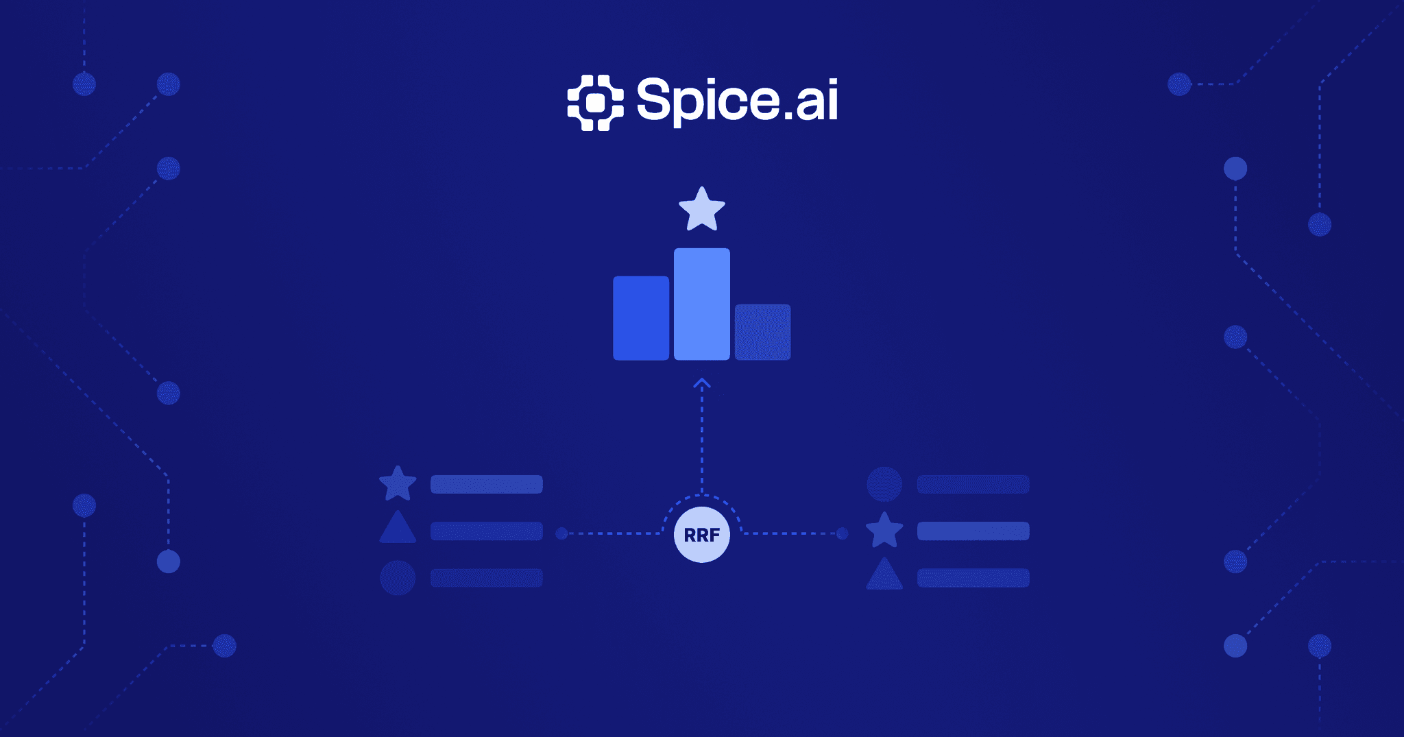
Neither method is strictly superior. Vector search excels at understanding intent and handling vocabulary mismatch. Keyword search excels at matching exact terms, identifiers, and technical terminology. In practice, hybrid search -- running both methods and fusing results with algorithms like Reciprocal Rank Fusion -- delivers the best results for most production use cases.

Vector Databases vs. Vector Search in SQL Engines

Teams implementing vector search have two architectural choices:

Dedicated vector databases (Pinecone, Weaviate, Qdrant, Milvus) are purpose-built for vector storage and search. They provide optimized ANN algorithms, built-in metadata filtering, and managed scaling. The tradeoff is another system to deploy, another data pipeline to maintain, and no native SQL support for joining vector results with relational data.

Vector search in SQL engines embeds vector indexing within a SQL-compatible query engine. This approach allows vector similarity search alongside standard SQL queries -- filtering, joining, aggregating -- in a single system. The tradeoff is that general-purpose SQL engines may not match the raw vector search performance of dedicated systems, though for most workloads the difference is negligible.

For RAG applications and enterprise AI use cases, the ability to combine vector search with SQL is a significant advantage. Filtering search results by metadata (date ranges, access permissions, document categories), joining with relational data, and expressing complex retrieval logic in SQL eliminates the application-layer glue code required when vector search and SQL live in separate systems.

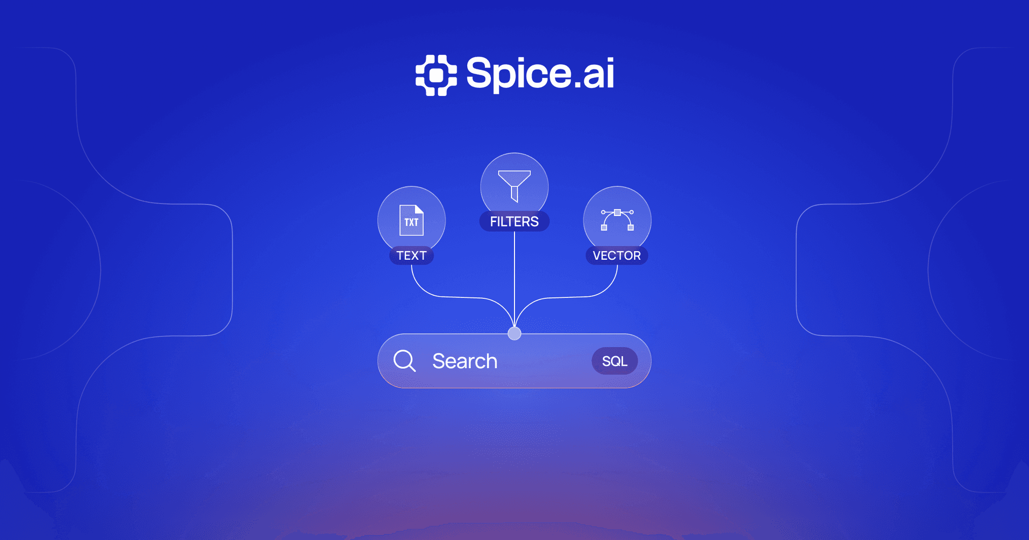
Vector Search with Spice

Spice provides vector similarity search alongside BM25 full-text search and SQL in a single unified runtime. This enables hybrid search -- combining vector and keyword results with built-in RRF fusion -- without managing separate systems.

Key capabilities:

• Vector, full-text, and SQL search in one query engine -- store embeddings, build vector indexes, and search alongside your relational data
• SQL federation across 30+ connected data sources, with vector search results joinable with federated data
• Real-time CDC to keep vector indexes fresh as source data changes
• LLM inference for generating embeddings alongside search queries in the same runtime

-- Vector similarity search in Spice
SELECT * FROM search(
  'knowledge_base',
  'how to optimize query performance',
  mode => 'vector',
  limit => 10
)

The unified approach eliminates the operational complexity of maintaining separate vector databases and keeping them synchronized with your primary data stores. When source data changes, both vector and keyword indexes update through the same change data capture pipeline, ensuring consistent search results across all modalities.

Advanced Topics

HNSW Internals

HNSW (Hierarchical Navigable Small World) constructs a proximity graph with a hierarchical structure inspired by skip lists. Understanding its internals helps with tuning:

Graph construction: When inserting a new vector, HNSW assigns it a random maximum layer (drawn from an exponential distribution). The vector is then connected to its nearest neighbors at each layer from the top down. The greedy search used during insertion finds these neighbors efficiently.

Key parameters:

• M: The number of bi-directional links per node at each layer. Higher M increases recall and memory usage. Typical values are 16-64.
• ef_construction: The size of the dynamic candidate list during index construction. Higher values produce a better graph (higher recall) at the cost of slower build times. Typical values are 100-400.
• ef_search: The size of the dynamic candidate list during search. Higher values increase recall at the cost of query latency. This is the primary parameter for tuning the recall-speed tradeoff at query time.

The relationship between these parameters is: ef_construction determines the quality ceiling of the graph, M determines the memory footprint, and ef_search controls the runtime tradeoff between recall and speed.

Filtered Vector Search

In practice, vector search rarely operates in isolation -- users want to filter results by metadata (date ranges, categories, access permissions) alongside semantic similarity. Filtered vector search combines vector nearest-neighbor queries with predicate-based filtering.

There are three approaches:

1. Pre-filtering: Apply metadata filters first, then search only the matching vectors. This is precise but can be slow if the filter is very selective (few matching vectors).
2. Post-filtering: Run vector search first, then filter results by metadata. This is fast but may return fewer than k results if many top candidates are filtered out.
3. Integrated filtering: Apply filters during the ANN search traversal. This is the most sophisticated approach, supported by modern vector indexes, and balances speed with precision.

The choice depends on filter selectivity. Highly selective filters (matching < 1% of documents) favor pre-filtering. Broad filters (matching > 50%) favor post-filtering or integrated filtering.

Multi-Vector Retrieval (ColBERT)

Standard vector search represents each document as a single embedding vector. ColBERT (Contextualized Late Interaction over BERT) takes a different approach: it represents each document as a set of token-level vectors (one per token) and computes similarity using late interaction.

At query time, each query token's vector is compared against all document token vectors using a MaxSim operation -- for each query token, find its maximum similarity to any document token, then sum these maximums. This token-level matching is more expressive than single-vector comparison because it can capture fine-grained relevance signals.

ColBERT achieves higher retrieval quality than single-vector models, especially on queries requiring precise term-level matching. The tradeoff is significantly higher storage requirements (one vector per token instead of one per document) and more complex index structures. Recent work on compressed ColBERT representations (ColBERTv2) reduces storage costs while maintaining most of the quality advantage.