Phillip has spent a decade building some of the largest distributed systems and big data platforms used by millions worldwide. Before co-founding Spice AI, Phillip was both an engineering manager and IC working on distributed systems at GitHub and Microsoft. Phillip has contributed to services developers use every day, including GitHub Actions, Azure Active Directory, and Visual Studio App Center.
\n', }, ], padding_top: 'unset', padding_bottom: 'unset', }} />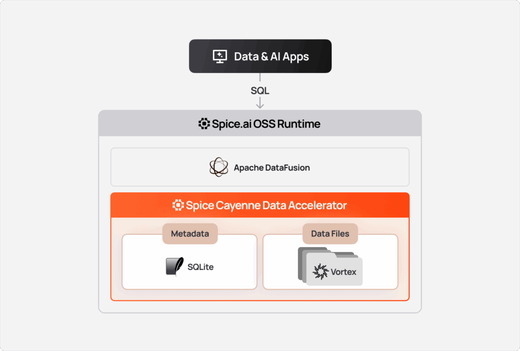
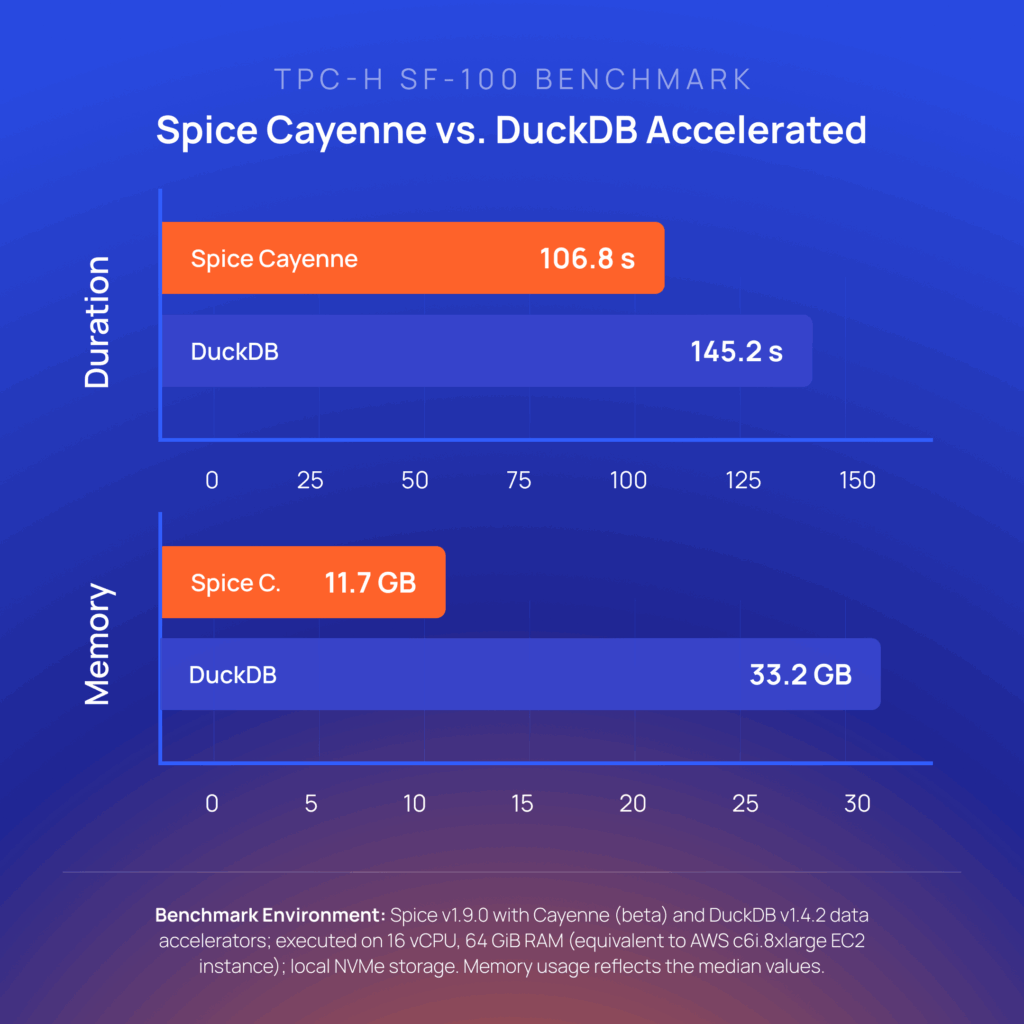
Spice Cayenne combines Vortex, the next-generation columnar file format from the Linux Foundation, with a simple, embedded metadata layer. This separation of concerns ensures that both the storage and metadata layers are fully optimized for what each does best. Cayenne delivers better performance and lower memory consumption than the existing DuckDB, Arrow, SQLite, and PostgreSQL data accelerators.' } />
additional_columns and where support for table relations in search, enabling multi‑table search workflows.
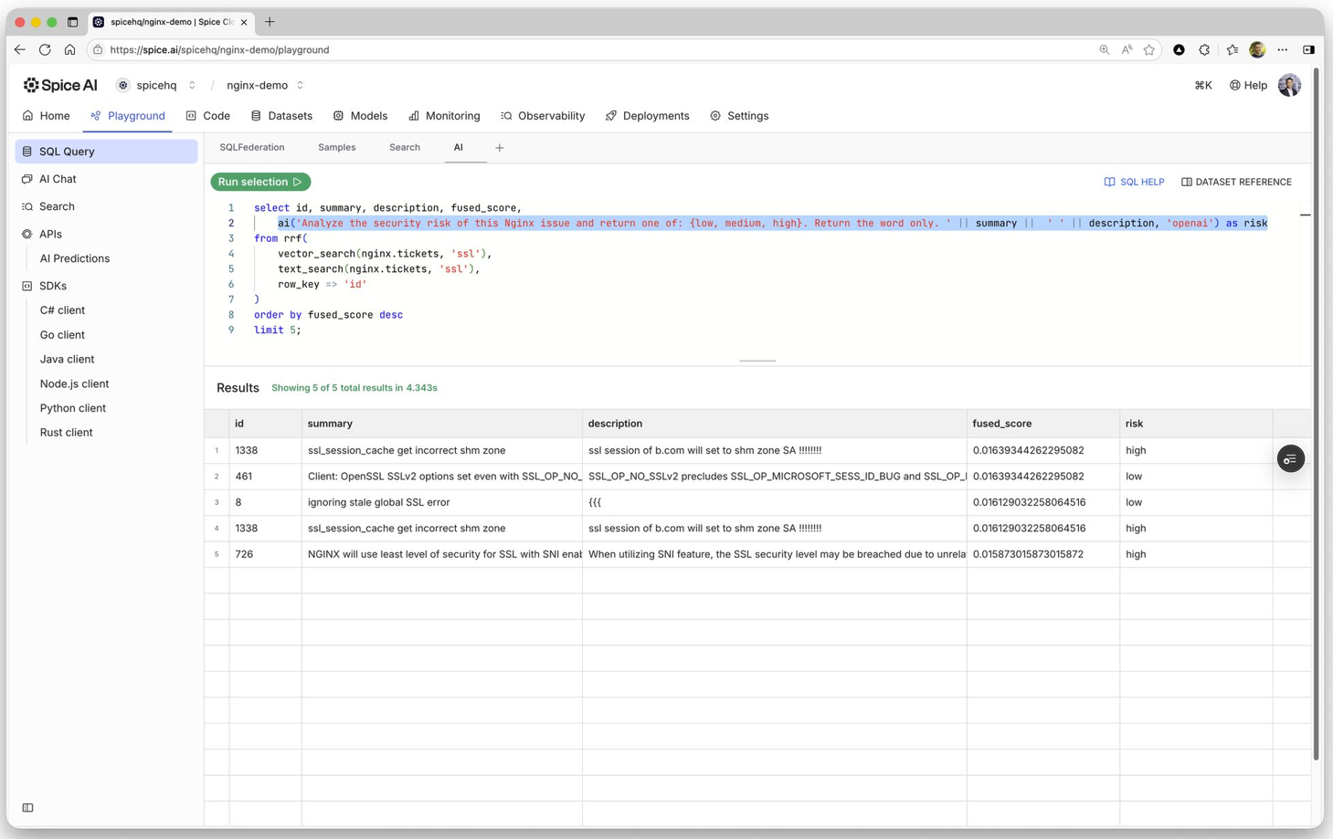
ai() SQL function enables developers to invoke LLMs directly within SQL for bulk generation, classification, translation, or analysis. Inference runs alongside joins, filters, aggregations, and search results without additional application-layer plumbing. Developers can transform federated data into structured insights extracting data, call external completion APIs, or orchestrate separate pipelines.'
}
/>
spicepod.yaml file with the following content: '
}
/>
```yaml
version: v1
kind: Spicepod
name: my_spicepod
datasets:
- from: s3://spiceai-demo-datasets/taxi_trips/2024/
name: taxi_trips
```
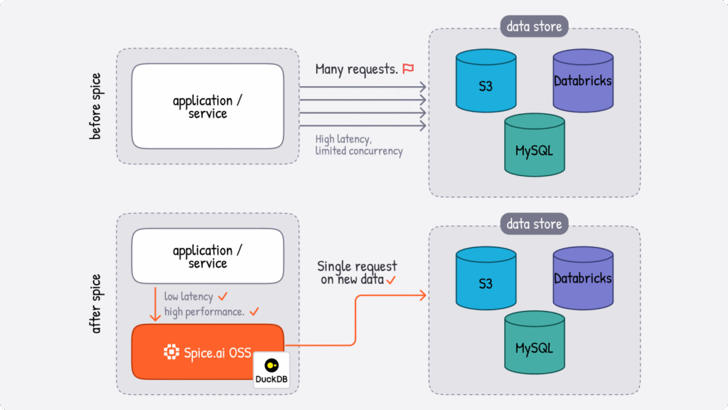
taxi_trips stored in a remote S3 bucket using standard SQL without copying or moving that data. That's federation in action - querying data where it lives, not where you've moved it to. "
}
/>
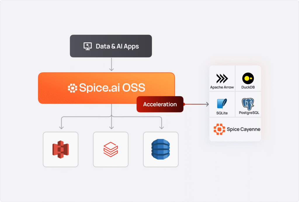
| Engine | Mode | Best For |
| Arrow | In-memory only | Ultra-fast analytical queries, ephemeral workloads |
| DuckDB | Memory or file | General-purpose OLAP, medium datasets, persistent storage |
| SQLite | Memory or file | Row-oriented lookups, OLTP patterns, lightweight deployments |
| Cayenne | File only | High-volume multi-file workloads, terabyte-scale data |
acceleration block to your dataset configuration: '
}
/>
```yaml
datasets:
- from: s3://data-lake/events/
name: events
acceleration:
enabled: true
engine: cayenne # Choose your engine
mode: file # 'memory' or 'file'
```
| Mode | Description | Use Case |
| full | Complete dataset replacement on each refresh | Small, slowly-changing datasets |
| append (batch) | Adds new records based on a time column | Append-only logs, time-series data |
| append (stream) | Continuous streaming without time column | Real-time event streams |
| changes | CDC-based incremental updates via Debezium or DynamoDB | Frequently updated transactional data |
| caching | Request-based row-level caching | API responses, HTTP endpoints |
Retention is particularly useful for time-series workloads like logs, metrics, and event streams where only recent data is relevant for queries. For example, an application monitoring dashboard might only need the last 7 days of logs for troubleshooting, while a real-time analytics pipeline processing IoT sensor data might retain just 24 hours of readings. By defining retention policies, you ensure accelerated datasets stay bounded and performant without manual intervention.
Spice supports two retention strategies: time-based, which removes records older than a specified period, and custom SQL-based, which executes arbitrary DELETE statements for more complex eviction logic. Once defined, Spice runs retention checks automatically at the configured interval: ' } /> ```yaml acceleration: # Common retention parameters retention_check_enabled: true retention_check_interval: 1h # Time-based retention policy retention_period: 7d # Custom SQL-based Retention retention_sql: "DELETE FROM logs WHERE status = 'archived'" ```
| Option | Description | Default |
cache_max_size | Entry expiration duration | 128 MiB |
item_ttl | Maximum cache storage | 1 second |
eviction_policy | `lru` (least-recently-used) or `tiny_lfu` | lru |
encoding | Compression: `zstd` or `none` | none |
refresh_complete: Creates snapshots after each refresh (full and batch-append modes) time_interval: Creates snapshots on a fixed schedule (all refresh modes) stream_batches: Creates snapshots after every N batches (streaming modes: Kafka, Debezium, DynamoDB Streams) spice chat CLI: '
}
/>
```bash
$ spice chat
Using model: gpt4
chat> How many orders were placed last month?
Based on the orders table, there were 15,234 orders placed last month.
```
/v1/nsql endpoint converts natural language to SQL and executes it: '
}
/>
```bash
curl -XPOST "http://localhost:8090/v1/nsql" \
-H "Content-Type: application/json" \
-d '{"query": "What was the highest tip any passenger gave?"}'
```
| Method | Best For | How It Works |
| Full-Text Search | Keyword matching, exact phrases | BM25 scoring via Tantivy |
| Vector Search | Semantic similarity, meaning-based retrieval | Embedding distance calculation |
| Hybrid Search | Queries with both keywords and semantic similarity | Hybrid execution and ranking through Reciprocal Rank Fusion (RRF) |
Spice supports both local embedding models (like sentence-transformers from Hugging Face) and remote providers (OpenAI, Anthropic, etc.). Embeddings are configured as top-level components and referenced in dataset columns:' } /> ```yaml datasets: - from: s3://docs/ name: documents vectors: enabled: true columns: - name: body embeddings: - from: openai_embed ``` ```sql SELECT * FROM vector_search (documents, 'How do I reset my password?', 10) WHERE category = 'support' ORDER BY score; ```
INSERT INTO statements. '
}
/>
read_write configuration.'
}
/>
| Deployment Model | Description | Best For |
| Standalone | Single instance via Docker or binary | Development, edge devices, simple workloads |
| Sidecar | Co-located with your application pod | Low-latency access, microservices architectures |
| Microservice | Multiple replicas deployed behind a load balancer | Loosely couple architectures, heavy or varying traffic |
| Cluster | Distributed multi-node deployment | Large-scale data, horizontal scaling, fault tolerance |
| Sharded | Horizontal data partitioning across multiple instances | Large scale data, distributed query execution |
| Tiered | Hybrid approach combining sidecar for performance and shared microservice for batch processing | Varying requirements across different application components |
| Cloud | Fully-managed cloud platform | Auto-scaling, built-in observability, zero operational overhead. |
| Concept | Purpose |
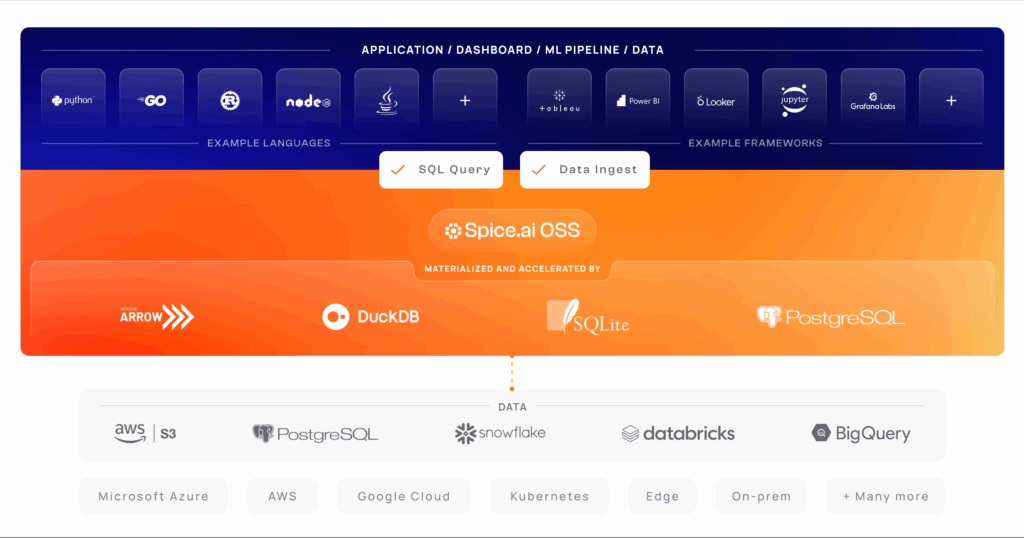
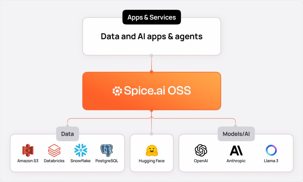
| Federation | Query 30+ sources with unified SQL |
| Acceleration | Materialize data locally for sub-second queries |
| Views | Virtual tables from SQL transformations |
| Snapshots | Fast cold-start from object storage |
| Models | Chat, NSQL, and embeddings via OpenAI-compatible API |
| Search | Full-text and vector search integrated in SQL |
| Writes | INSERT INTO for Iceberg and Amazon S3 tables |
| Use Case | How Spice Helps |
| Operational Data Lakehouse | Serve real-time operational workloads and AI agents directly from Apache Iceberg, Delta Lake, or Parquet with sub-second query latency. Spice federates across object storage and databases, accelerates datasets locally, and integrates hybrid search and LLM inference - eliminating separate systems for operational access. |
| Data lake Accelerator | Accelerate data lake queries from seconds to milliseconds by materializing frequently-accessed datasets in local engines. Maintain the scale and cost efficiency of object storage while delivering operational-grade query performance with configurable refresh policies. |
| Data Mesh | Unified SQL access across distributed data sources with automatic performance optimization |
| Enterprise Search | Combine semantic and full-text search across structured and unstructured data |
| RAG Pipelines | Merge federated data with vector search and LLMs for context-aware AI applications |
| Real-Time Analytics | Stream data from Kafka or DynamoDB with sub-second latency into accelerated tables |
| Agentic AI | Build autonomous agents with tool-augmented LLMs and fast access to operational data |